from model import JML_trainer
from util import standardize_V_Z_U_promax

Y_missing = torch.load("data/Y_matrix.pt")
train_mask, test_mask = random_mask((Y_missing != -1).float(), pct=0.8)
model_FA = JML_trainer(Y_missing, K=4, mask=train_mask, device="cuda:0", is_map=True)

V, Z, U = standardize_V_Z_U_promax(model_FA.U, model_FA.V, model_FA.Z)4 Generalization
Large language models (LLMs) are often evaluated by running them on benchmarks and asking an AI judge to score their answers.
However, judging introduces bias and high cost — each (model, question) pair must be queried and scored.
This tutorial walks through an alternative framework — Prediction-Powered Evaluation (PPE) — which predicts correctness without running models or judges.
It combines factor analysis and semantic prediction to estimate correctness probabilities for unseen questions or unseen models.
4.1 Motivation
4.1.1 Limitations of Judge-Based Evaluation
Judge-based approaches are expensive and biased by surface-level style features (e.g., bulleting, verbosity).
We formalize two approaches to measuring correctness:
\[ p_\theta(Y_{ij}=1 \mid i,j,D_{\text{train}}) = \sigma(H_{ij}(\theta)) \]
and the judging variant:
\[ p_\theta(Y_{ij}=1 \mid i,j,k,D_{\text{train}}) = \mathbb{E}_k[p_\theta(Y_{ij}=1 \mid i,j,k,D_{\text{train}})] \]
Let \(S\) denote style (e.g., response length).
Then the judge model induces a bias pathway \(S \to R \to \hat Y_{\text{judge}}\),
while the prediction-powered correctness model \(\hat Y_{\text{corr}}\) remains unbiased:
\[ \text{Bias}_{\text{judge}}(s) = E[\hat Y_{\text{judge}} - Y^* \mid S=s], \quad \text{Bias}_{\text{corr}}(s) = 0. \]
This framework enables cost-efficient, style-invariant evaluation, avoiding the stylistic confounds of AI judges.
4.1.2 The Hardness of Mapping from Semantics to Behavior
Even if we could perfectly represent question meaning, semantic similarity does not guarantee behavioral similarity.
Two questions that appear linguistically close may elicit very different correctness patterns across models.
We compare:
- Semantic similarity: cosine similarity between question embeddings
- Behavioral similarity: tetrachoric correlation between model responses
\[ \text{Corr}_{\text{semantic}}(i,j) = \cos(E_i, E_j), \quad \text{Corr}_{\text{behavioral}}(i,j) = \text{TetraCorr}(Y_{\cdot i}, Y_{\cdot j}) \]
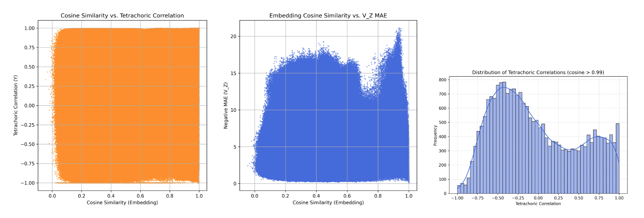
As shown in Figure 4.1,
there is no consistent relationship between these two measures — even when \(\cos(E_i, E_j) > 0.99\),
the behavioral correlation can range from −1 to +1.
This randomness reveals that semantic embeddings are poor instruments for explaining or predicting response behavior.
Observation: Semantically similar questions (cosine > 0.99) exhibit nearly random behavioral correlations (−1 to +1),
showing that linguistic proximity does not imply behavioral equivalence.
4.2 Stage 1 — Factor Model Pretraining
We first learn latent behavioral factors \((U, V, Z)\) from response data \(Y_{ij}\).
\[ p(Y_{ij}=1 \mid U_i, V_j, Z_j) = \sigma(U_i^\top V_j + Z_j) \]
Each model \(i\) has latent ability vector \(U_i\), and each question \(j\) has parameters \(V_j\) and difficulty bias \(Z_j\).
The factor model captures the behavioral structure of models across benchmarks and serves as the foundation for prediction.
4.3 Stage 2 — Prediction-Powered Correctness Model
The next step learns to predict behavioral parameters directly from metadata and semantics, without observing responses.
Two parallel predictors are trained:
- Item-side predictor \(f_V\): maps question embeddings to \((\hat V_j, \hat Z_j)\)
- Model-side predictor \(f_U\): maps model features to \(\hat U_i\)
These predictors allow cold-start evaluation, predicting new entries in the response matrix \(Y\).
4.3.1 Predicting Item Embeddings from Question Semantics
We train a neural network to map question embeddings \(E_j \in \mathbb{R}^{4096}\) to latent parameters:
\[ [\hat V_j, \hat Z_j] = f_\theta(E_j) \]
from model import embedding_V
from torch.distributions import Bernoulli

K = 4
model_V = embedding_V(input_dim=4096, output_dim=K+1).to(device)
optimizer = torch.optim.Adam(model_V.parameters(), lr=1e-3)

for epoch in range(2000):
pred = model_V(E_train)  # [n_items, K+1]
pred_V, pred_Z = pred[:, :K], pred[:, K:]
probs = torch.sigmoid(U @ pred_V.T + pred_Z.T)
loss = -Bernoulli(probs=probs[train_mask]).log_prob(Y[train_mask].float()).mean()
optimizer.zero_grad(); loss.backward(); optimizer.step()
The loss minimizes the Bernoulli log-likelihood using fixed \(U\) from the factor model.
4.3.2 Predicting Model Embeddings from Metadata
Each model has a 24-dimensional feature vector describing its scale, architecture, and release time.
We fit a linear transformation to predict \(U\):
\[ \hat U_i = f_\phi(F_i) = F_i W_U \]
This simple mapping encourages interpretability and stable convergence.
4.4 Stage 3 — Cold-Start Evaluation
Once we have learned both mappings, we can reconstruct correctness probabilities:
\[ \hat P_{ij} = \sigma(\hat U_i^\top \hat V_j + \hat Z_j) \]
and evaluate on unseen rows or columns of \(Y\).
Typical results:
| Split | AUC |
|---|---|
| randcol–randcol | 0.804 |
| randrow–randrow | 0.848 |
These confirm that the semantic–behavioral mapping generalizes well.
4.5 Mapping Semantic to Behavioral Space
To study whether semantically similar questions behave similarly,
we compute cosine similarity of question embeddings and tetrachoric correlation of their responses.
from util import tetrachoric_matrix_torch
import seaborn as sns, matplotlib.pyplot as plt

R = tetrachoric_matrix_torch(Y)
cosine = torch.corrcoef(V.T)

sns.scatterplot(x=cosine.flatten(), y=R.flatten(), s=5, alpha=0.5)
plt.xlabel("Cosine Similarity (semantic)")
plt.ylabel("Tetrachoric Correlation (behavior)")
plt.title("Semantic vs Behavioral Similarity")
Observation: Even highly similar questions (cosine > 0.99) exhibit nearly random behavioral correlations (−1 to +1),
showing that semantic proximity is a poor instrument for behavioral prediction.
4.6 Iterative Filtering via Tetrachoric Correlation
We remove inconsistent or adversarial items via iterative filtering.
After 19 rounds:
- Retained: 11,243 of 20,743 questions (~54%)
- Negative correlations: ↓ from 23% → 1.67%
- Benchmark composition: stable across iterations
This step improves inter-item consistency and downstream factor modeling.
4.7 Generalization to New Models
We evaluate generalization to unseen models under the randrow–randrow split.
Predict \(U_{test}\) from metadata and evaluate:
Result:
AUC ≈ 0.8483 with \(K = 1\), confirming strong linear predictability of model behavior from simple metadata.
4.8 Summary of the Prediction-Powered Framework
| Component | Input | Output | Purpose |
|---|---|---|---|
| Factor model | Response matrix \(Y\) | \(U, V, Z\) | Extract latent behavior |
| Semantic predictor | Question embeddings \(E_j\) | \([\hat V_j, \hat Z_j]\) | Generalize to unseen questions |
| Model predictor | Metadata \(F_i\) | \(\hat U_i\) | Generalize to unseen models |
| Correctness predictor | \(\hat U_i, \hat V_j, \hat Z_j\) | \(\hat P_{ij}\) | Predict correctness without judging |
This pipeline allows reliable, low-cost, and bias-resistant measurement of model performance under cold-start conditions.
4.9 Implications
- Efficiency: Predicts correctness for new benchmarks without running any model queries.
- Reliability: Invariant to stylistic confounds.
- Scalability: Cost scales as \(O(N + M)\) instead of \(O(NM)\).
- Interpretability: Latent factors preserve behavioral semantics for explainable evaluation.
This tutorial is based on the paper “Measuring Without Judging: Prediction-Powered Cold-Start Evaluation” (Anonymous, 2025).
It demonstrates how factor models, semantic mapping, and adaptive filtering jointly enable a new paradigm of scalable AI evaluation.